5.18. Obtaining MC distributions and statistics derived of it in detail

During the Monte Carlo simulation successively three different distributions are produced from which some statistics are derived. The latter are the arithmetic mean, the standard deviation of the distribution and especially certain quantiles.

At the beginning the (large) number N of simulated measurement values of the output quantity is defined. This defines one “run”. Several runs (number r; maximum 50) may be calculated which then allows statistical evaluations to be made of the statistics mentioned above; from the r-fold repetition of the simulation one gets for instance with the standard deviation of the r values of a statistic an indication of its uncertainty.

Determining a quantile

The MC procedure use previously was primarily designed for nearly symmetric distributions of the output quantity. With applying more and more the GUM Supplement 1 with asymmetric distributions of some specific input quantities may result in a rather asymmetric distribution of the output quantity. Extreme values, to be expected for the distribution, had to be fixed in the program in advance, which turned out to be a disadvantage.

Therefore, with version 2.1.9 the MC procedure was modified – and thereby simplified, in that all MC values of the output quantity are now store in an array. Now, for every of the three above mentioned distributions MC simulation yields arrays of up to 2 000 000 MC values. From these arrays mean and standard deviation are easily calculated. Quantiles are estimated by a distribution-free method, which requires sorting the arrays first. Only for the purpose of graphical representation as a histogram, the MC values have to be sorted into 20 000 Bins („multi-channel“); the limits of the histograms are determined after the MC simulation – and not before. These modifications made the MC procedure code easier to handle.

1. Bayesian estimates

For the estimation of mean, standard deviation and lower and upper confidence limits according to the Bayesian method only the distribution truncated at zero is used, values below zero are not used and not considered for the total number of values. The confidence limits are estimated as lower and upper quantile of the distribution. The total number of values considered in one run is only about N/2.

With Version 1.03 an option was added within the dialog „Results“, MC section, with which it is possible to calculate a special pair of coverage limits which has the shortest distance (Bayesian coverage interval of shortest length) instead of the symmetrical confidence limits. Test case: Neutron-Dose-Cox-2006_EN.txp. The activation of this option does not lead to a significant increase of simulation duration.

Input parameters being associated with an asymmetric or rectangular distribution may result in a significant asymmetry of the output quantity distribution. In the decision threshold case this may cause some deviation of the mean value from zero.

At first, a deviation from an expected distribution symmetrically to zero is tested. This is done by comparing the mean value y₁, deviating from zero, with the MC uncertainty of the mean, u(y₁)/√N (see below). In the case of

\(\frac{y_{1}}{u\left( y_{1} \right)/\sqrt{N}} > 0.10\ \)

an iteration is performed for the decision threshold using the secant method, which shifts the mean value closer to zero. If necessary, up to 12 steps are performed, each of them requiring a full MC simulation; this leads to increasing computational effort. If the above ratio does not fall below 0.10, that distribution with the lowest ratio is selected from those of the 12 steps, from which the decision threshold is then calculated. y₁ can be reduced by typically one to two orders of magnitude; it may happen, however, that y₁ is reduced by hardly more that a factor of 10.

2. Decision threshold

For the estimation of the Decision threshold a modification is applied which consists of setting the “true value” of the net counting rate (thereby also of the activity) equal to zero. This results in a distribution which to about 50 % has negative values. In this case, no truncation at zero is applied. The upper (1-\(\alpha\)) quantile of this distribution represents the simulated value of the Decision threshold.

3. Detection limit

The estimation of the Detection limit is the most time-consuming part of the simulation, because in this case the distribution is shifted several times by changing the mean of the distribution, each time after the total number N is reached. The aim of the step-wise shifting hereby is that the (lower) ß Quantile of this distribution has to come as close to the value of the Decision threshold (determined before, see above) as possible. This iteration procedure is based on a bi-section method but with dividing the interval by linear interpolation.

Negative values are explicitly considered in these calculations.

The motivation not to discard negative parts of the distributions for the estimation of Decision threshold and Detection limit comes from the fact that the primary result for the output quantity shall be directly comparable with Decision threshold. If the negative parts would be discarded, a transformation being in analogy to the truncation would have to be applied to the primary output quantity before such a comparison

To make the distributions non-negative in the case of the Bayesian estimates is possible after a comparison between primary output quantity and the Decision limit has been done and has led to the conclusion that the assumption of a non-zero activity value in the sample is true.

Estimating the MC uncertainties of the characteristic values

Performing a MC-Simulation with only one single run did up to now not give any estimates of the uncertainties associated the characteristic values. Furthermore, when using a small number of runs, the estimates obtained from the spreading within the runs also are not very reliable.

As the resulting MC distributions in most cases are normal distributions, uncertainties of characteristic values can be roughly estimated as follows (see e.g. Barlow, 1999):

Characteristic value:	Width parameter:	Formula for the (absolute) uncertainty:
Value of output quantity	\(\sigma\)	\(\frac{\sigma}{\sqrt{N}}\)
Uncertainty	\(\sigma\)	\(\frac{\sigma}{\sqrt{2N}}\)
Lower confidence limit	\(\sigma\)	\(\frac{\sigma}{\varphi\left( \Phi^{-1}(1 - \gamma/2) \right)}\sqrt{\frac{(1 - \gamma/2) \cdot \gamma/2}{N}}\)
Upper confidence limit	\(\sigma\)	dito
Decision threshold	\(\sigma^* = \frac{y^*}{k_{1 - \alpha}}\)	\(u_{MC}\left( y^{*} \right) = \frac{\sigma^*}{\varphi\left( \Phi^{-1}(1 - \alpha) \right)}\sqrt{\frac{(1 - \alpha) \cdot \alpha}{N}}\)
Detection limit	\(\sigma^{\#} = \frac{y^{\#} - y^*}{k_{1 - \beta}}\)	\(u_{MC}\left( y^{\#} \right) = \sqrt{u_{MC}^{2}\left( y^{*} \right) + u^{\#\ 2}}\), with \(u^{\#} = \frac{\sigma^{\#}}{\varphi\left( \Phi^{-1}(1 - \beta) \right)}\sqrt{\frac{(1 - \beta) \cdot \beta}{N}}\)

(N: number of MC-simulated single measurements; ϕ(.) and Φ(.): density function and distribution function of the standard normal distribution, respectively; see Options dialog for the probabilities α, β and γ).

The MC uncertainties calculated according to this table are given as relative values in percent within the MC part under the TAB „Results“, but only in the case of one single run.

Graphical presentations

The distributions which are produced according to the three methods discussed above are displayed as histograms in a separate window while the simulation is running. They show each distribution accumulated from the r runs which stabilize after only few (of r) repetitions. In the case of the Detection limit the accumulated distribution is displayed after the r runs are terminated. The x-axis (abscissa) corresponds to values of the evaluated quantity shown in the title of a plot; the y-axis (ordinate) shows the probability.

Example of the separate window with the MC graphs:

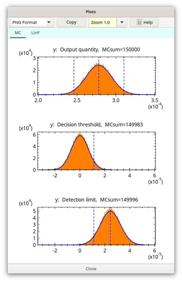
Vertical green lines in the graphs characterize, from the left to the right, the following values:

distribution of: values:

output quantity lower confidence limit, best estimate (Bayesian), upper confidence limit

Decision threshold its value

Detection limit Decision threshold, Detection limit

After each single MC run that Gaussian curve is potted in blue color which corresponds to the result of the analytical procedure.

Note: The separate window with the MC graphs is maintained after completion of the MC simulation calculations. This allows for additional inspection of data shown under the different TABs and for invoking a result report and to go then back to “Results” TAB with this window. If data or options were changed during this step having the consequence that the original assumptions underlying the MC simulation are no longer valid, this MC window will be closed. This is also done when again calculations in the TAB “Values, Uncertainties” or calculations initiated by the change from TAB “Values, Uncertainties” to the TAB TAB “Uncertainty Budget” are invoked.