
4.4. Utilizing a calibration curve
There were demands existing to consider within an evaluation a specific input quantity (e.g. the detection efficiency) as being dependent on “another” quantity (such as area mass density, or a quench factor), which means to take its value from an associated “calibration curve” by interpolating a polynomial function of the “other” quantity.
For this purpose, a new function KALFIT was established, for which a new dialog allows input of values x(i) and y(i) together with their standard uncertainties. x and y (independent and dependent variables, respectively) represent measured values of a calibration curve. The curve is modeled by a polynomial with maximum degree of 3 (max 4 coefficients). The polynomial coefficients are calculated by a weighted or non-weighted (multi-) linear least squares fit.
Unused (empty) columns in this dialog’s grid are set internally equal to 1.
Choosing a polynomial degree of 0 (i.e. 1 coefficient to be fitted), fitting of the y-values results in a weighted mean (uncertainties given) or in a non-weighted mean (uncertainties not given). Its standard uncertainty is that of the mean, i.e. already divided by the square root of the number of values.
Activating the calibration curve tool:
In this example KALFIT is called to determine the detection efficiency value eps (and its uncertainty) as a function of a quench factor eskv by using the fitted polynomial for interpolation.
The second parameter (i.er., eskv) represents a value of the independent quantity X, by which value and standard uncertainty of the dependent quantity Y (in this case of eps) are determined.
The first parameter of this function (here: 1) gives the information
about how to use the calibration curve for calculating the value of the
left side of Eq. (4.4.1) The value 1 means that the value for Y is
calculated (read) as polynomial just as shown above. The value 2 means
that the value for Y is determined by reversing the polynomial. An
example for the latter case is treated in the UR project
Example_8_with_KALFIT_EN.txp, for which the Eq. (4.4.1) above is replaced
by:
It means that Rnet designates count rates, which in a first step are calibrated as polynomial function dependent on known concentration values x: Rnet = Polynomial(x). The second step is to measure a count rate Rnetx of another sample and to determine then its associated concentration Cx. Assuming a degree 1 of the polynomial one would calculate the concentration Cx by (Rnetx-a1)/a2; for a higher-degree polynomial a numerical bisection method is used for the inversion. In the mentioned UR project, the concentration refers to that of Potassium given in g/L.
This KALFIT call invokes a new dialog (there is also a new item under the main menu Edit), by which the x- and y-values of such a calibration curve (including their standard uncertainties) can be input; the desired value for eps is taken via its x-value eskv from the polynomial curve for the y-values. Another button allows executing the polynomial fitting (max. degree of polynomial = 3) such that the final value and the standard uncertainty are made available to UR for the quantity eps.
The standard uncertainty of the desired Y-value (eps) is calculated by numerical uncertainty propagation using the fitted parameters \(a_{i}\) and their covariance matrix and the uncertainty of the given x-value \(x_{0}\) (eskv).
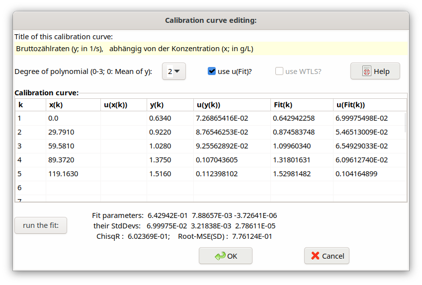
Fig. 4.4.1 KALFIT example
Although eps – as defined by the equation above – formally is a dependent quantity, it is treated in UR as if it were an independent quantity, e.g. regarding the uncertainty budget.
Currently, UR assumes that the value of only one input quantity is determined by a call to KALFIT.
The uncertainties of the x-values are currently not considered.
The following dialog shows an example of calculating a mean value (degree of polynomial equal to zero); the values to averaged are always the ones in the column for y(i).
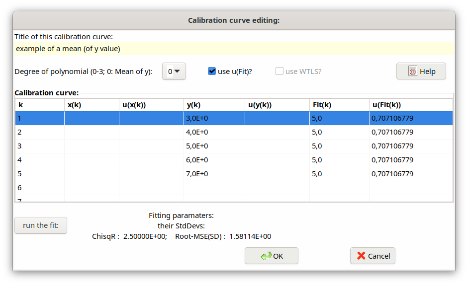
Fig. 4.4.2 Example mean value from KALFIT
