4.8. Confidence ellipses

Confidence ellipses are invoked from the main menu item “Options – Calculate confidence ellipse”.

Construction of the ellipse

The construction of a confidence ellipse of a pair of output quantities is outlined following the GUM Supplement 2 as follows.

At first the covariance matrix Uy of two output quantities is determined. For the latter, designated here as y₁ und y₂, their covariance matrix Uy consists of the diagonal elements \(u^{2}\left( y_{1} \right)\) and \(u^{2}\left( y_{2} \right)\) and of the identical non-diagonal elements \(\rho\ u\left( y_{1} \right)u\left( y_{2} \right)\), with their correlation coefficient \(\rho\).

For the lower triangular matrix L of a Cholesky decomposition of Uy, indicated by Uy=L L^T, the eigenvalues d are calculated by the Jacobi method.

The length values a of the semi-axes of the ellipse and the angle θ between the axes of the ellipse and the axes of the coordinate system are derived from the equations

\(a_{j} = \sqrt{d_{j\ }\chi_{(1 - \gamma);2}^{2}}\) , j =1,2

\(\theta = {\frac{1}{2}\tan}^{- 1}\left( \frac{2\rho\ u\left( y_{1} \right)u\left( y_{2} \right)}{u^{2}\left( y_{1} \right) - u^{2}\left( y_{2} \right)} \right)\)

where \(\chi_{(1 - \gamma);2}^{2} = 5.99146\) is the (1-γ) quantile of the Chi-square distribution with 2 degrees of freedom.

Graphical realization

The following figure shows such a confidence ellipse in the left graph. This does not yet correspond with our knowledge of an ellipse, because their principal axes are not vertical. This behavior originates in different scaling units of the two coordinate axes; e.g. 5 scale units show quite different lengths.

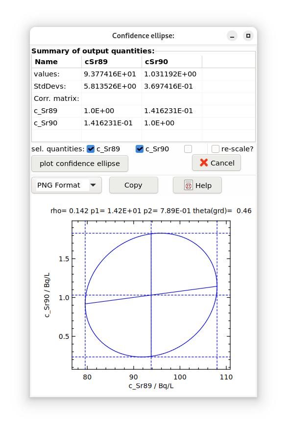
Fig. 4.8.1 both axes have different scales

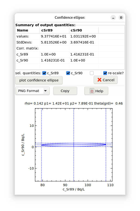
Fig. 4.8.2 re-scale: both axes have the same scale (5 scale units have the same length on both axes)

This disadvantage can be removed by introducing the same scale for both axes. This can be achieved by the following re-scaling (in the GUM Supplement 2 it was prevented to use different scaling):

\(u\left( y_{1} \right)\ \leq u\left( y_{2} \right)\) : \(y_{1} \rightarrow y_{1}\frac{u\left( y_{2} \right)}{u\left( y_{1} \right)}\) ,

or

\(u\left( y_{2} \right)\ \leq u\left( y_{1} \right)\) : \(y_{2} \rightarrow y_{2}\frac{u\left( y_{1} \right)}{u\left( y_{2} \right)}\) .

For a graphical presentation the points of the ellipse curve are at first calculated by assuming that the origin of the ellipse is identical with the origin of the coordinate system and that the angle between the axes of the ellipse and of the coordinate system is zero. Applying then a coordinate transformation, consisting of the two operations of a translation and a rotation, are then moved to the final curve of the ellipse which is plotted then.

The right-hand graph of the Figure shown above displays the re-scaled ellipse; their semi-axes are now perpendicular. Within both graphs, the intervals

\(y_{j} \pm u\left( y_{j} \right)\sqrt{\chi_{(1 - \gamma);2}^{2}}\)

are indicated as dotted lines.

Literature:

JCGM 102:2011 (GUM Supplement 2, 2011)

Brandt, S., 1999, Kapitel 5.10 und A.12

Press et al., 1992, chapter 11.1

13. 1. Thompson, 2015: Gaussian Statistics Lecture

23. 5. Hoover, 1984